67 forcats and factors

Written by Matthew Wankiewicz and last updated on 7 October 2021.

67.1 Introduction

In this lesson, you will learn about:

Factors in R, how they work, what they do.
The forcats package.

Highlights:

Factors are a way of storing data in R. Instead of having many different combinations like a list of names or numbers, factors are usually created to represent a fixed number of values, such as levels (high, low, medium) or times (early, late, on-time). In other words, factors represent categorical data in R.
forcats contains many functions that allow you to work with factors for plotting or further data analysis.

67.2 The Content

Factors represent categorical variables in R. Factors are stored as integer levels in R, meaning that each level of a factor will be represented by an integer so R knows which one represents the maximum and minimum. Factors can be comprised of both integers and characters but the levels of these factors will be displayed as characters. The factor function can be used to create factors in R, it takes a vector of data and will turn it into a factor. This function can be used on columns in datasets to convert a column of data from numeric/character to a factor.

forcats is a package that contains various functions to manipulate factors, it exists as its own package but is also included in the tidyverse package as well. The main goals of these functions are to help reorder and change factor levels, this is done by changing which levels appear at the front/back and also combining levels into other ones.

A helpful cheatsheet for forcats can be found here.

67.3 Factors

The factor function allows you to take a vector and turn it into a factor. The vector used can be made up of characters or integers. Its main argument is the vector that you want to turn into a factor. An example of this is shown below.

factor_vector <- c(1,2,3)
factor(x = factor_vector)
#> [1] 1 2 3
#> Levels: 1 2 3

In addition to the main argument, factor also has some optional arguments. These include levels, labels and exclude. levels tells R what the order of the levels are of your factor (which is highest/lowest), if you leave it empty it will make the levels in alphabetical order or increasing order for integers. labels will create labels for your factor and will set the order of your factor. exclude will take out a level that appears in your factor and replace those values with <NA>.

We can change the levels of our factor_vector from earlier using the levels argument.

factor_vector <- c(1,2,3)
factor(x = factor_vector, levels = c(2,1,3)) ## set levels to 2,1,3
#> [1] 1 2 3
#> Levels: 2 1 3

Using the labels argument, we can rename the levels of factor_vector. This will rename 1 to ‘one,’ 2 to ‘two’ and 3 to ‘three.’

factor_vector <- c(1,2,3)
factor(x = factor_vector, labels = c('one', 'two', 'three')) ## set labels to 'one', 'two', 'three'
#> [1] one   two   three
#> Levels: one two three

Using exclude we can exclude the number two from our factor.

factor_vector <- c(1,2,3)
factor(x = factor_vector, exclude = 2)
#> [1] 1    <NA> 3   
#> Levels: 1 3

If you want to test if a column or set of data is a factor, you can use is.factor.

factor_vector <- c(1,2,3)
new_factor <- factor(x = factor_vector, exclude = 2)

is.factor(x = new_factor)
#> [1] TRUE

You can also check the levels of a factor using levels

factor_vector <- c(1,2,3)
new_factor <- factor(x = factor_vector)

levels(x = new_factor)
#> [1] "1" "2" "3"

67.4 Forcats

There are many useful functions in the forcats library but this lesson will mainly focus on fct_relevel and fct_reorder while also looking briefly at fct_count, fct_c and fct_lump.

67.4.1 `fct_count`

This function can be used to count the number of values in each level of your factor. It takes one main argument, the factor you want to count. The other optional arguments (sort, prop) sort the most common levels to the top and can compute the proportion of the levels represented.

random_factor <- factor(x = c(1,1,1,2,3,4,2,3,2,1,4,3,3,3,2,1))
fct_count(random_factor)
#> # A tibble: 4 × 2
#>   f         n
#>   <fct> <int>
#> 1 1         5
#> 2 2         4
#> 3 3         5
#> 4 4         2

fct_count(random_factor, sort = TRUE)
#> # A tibble: 4 × 2
#>   f         n
#>   <fct> <int>
#> 1 1         5
#> 2 3         5
#> 3 2         4
#> 4 4         2

fct_count(random_factor, sort = TRUE, prop = TRUE)
#> # A tibble: 4 × 3
#>   f         n     p
#>   <fct> <int> <dbl>
#> 1 1         5 0.312
#> 2 3         5 0.312
#> 3 2         4 0.25 
#> 4 4         2 0.125

67.4.2 `fct_c`

This function takes factors with different levels and can combine them into one factor with the levels from the other factors. The only argument it takes are the factors you want to combine. We see that when using it on factors with levels ‘a’ and ‘b’ it will combine them into one factor with levels ‘a’ and ‘b.’

factor_a <- factor(x = "a")
factor_b <- factor(x = "b")

fct_c(factor_a, factor_b)
#> [1] a b
#> Levels: a b

67.4.3 `fct_lump` functions

This group of functions takes levels and brings them together to form a level called “other.” The functions include:

fct_lump_min: This function takes a factor and a number which tells R whether to include the level in other. An optional argument is called other_level, this will change the name of the “other” level.
fct_lump_prop: This function will lump levels that appear less than a certain proportion of times. For example, you can lump functions that make up less than 15% of your data.
fct_lump_n: This function lumps all of the levels except the n most frequent ones.

random_factor <- factor(x = c(1,1,1,2,3,4,2,3,2,1,4,3,3,3,2,1,1))

fct_lump_n(random_factor, n = 2) # keep the 2 most frequent levels
#>  [1] 1     1     1     Other 3     Other Other 3     Other
#> [10] 1     Other 3     3     3     Other 1     1    
#> Levels: 1 3 Other
fct_lump_prop(random_factor, prop = .25) # lump levels which appear less than 25 % of time
#>  [1] 1     1     1     Other 3     Other Other 3     Other
#> [10] 1     Other 3     3     3     Other 1     1    
#> Levels: 1 3 Other
fct_lump_min(random_factor, min = 3) # lump levels which appear less than 3 times
#>  [1] 1     1     1     2     3     Other 2     3     2    
#> [10] 1     Other 3     3     3     2     1     1    
#> Levels: 1 2 3 Other

67.4.4 `fct_reorder`

This function is useful when working with factors because it allows you to reorder a factor you are working with by another variable. For example, you can reorder a factor with levels of different sports by the average height for the sports listed. The first argument for this function is the factor/variable you plan to re-order and the second will be the variable you are sorting the factor by.

Using the expeditions data which looks at Himalayan expeditions, we can reorder the levels of the seasons by the average peak height for each season. As you can see, by adding the mutate line we can change the order of the levels depending on the mean height reached that season.

data_ex <- expeditions %>% 
  group_by(season) %>% 
  summarise(mean_height = mean(highpoint_metres, na.rm = T))

data_ex %>% 
  ggplot(aes(x = season, y = mean_height)) +
  geom_col() +
  labs(title = "Plot without fct_reorder")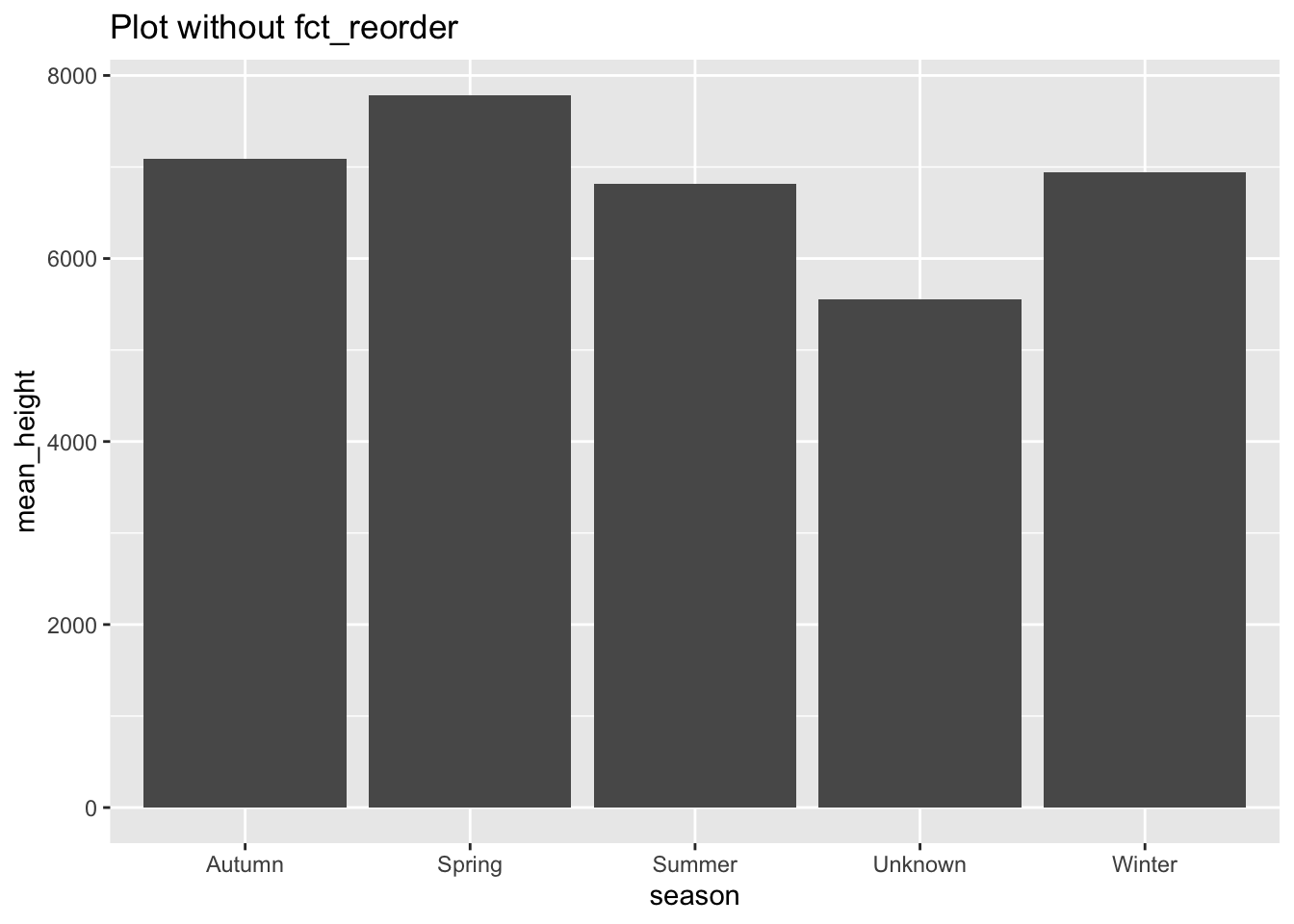


data_ex %>% 
  mutate(season = fct_reorder(season, mean_height)) %>% 
  ggplot(aes(x = season, y = mean_height)) +
  geom_col() +
  labs(title = "Plot with fct_reorder")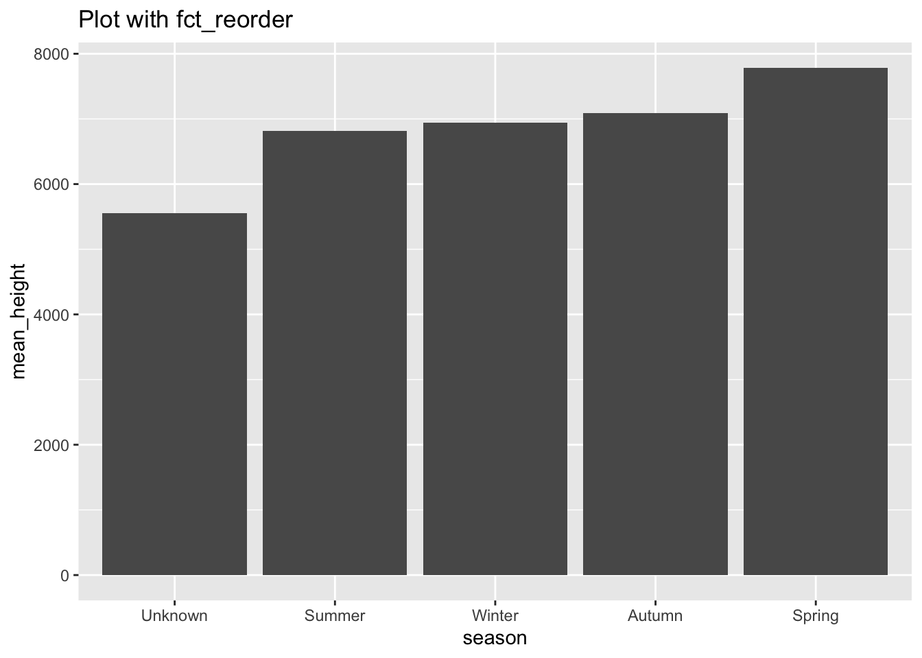


data_sorted <- data_ex %>% 
  mutate(season = fct_reorder(season, desc(mean_height)))

levels(as.factor(data_ex$season))
#> [1] "Autumn"  "Spring"  "Summer"  "Unknown" "Winter"
levels(data_sorted$season)
#> [1] "Spring"  "Autumn"  "Winter"  "Summer"  "Unknown"

We can see that the original order was alphabetical while the new sorted one is not.

fct_reorder can also be used to sort factors in descending order. We will use the same dataset, but this time we will order the levels of seasons decreasing by number of staff hired

crew_group <-expeditions %>% 
  group_by(season) %>% 
  summarise(mean_staff = mean(hired_staff, na.rm = T))

crew_group %>% 
  ggplot(aes(x = season, y = mean_staff)) +
  geom_col() +
  labs(title = "Plot without fct_reorder")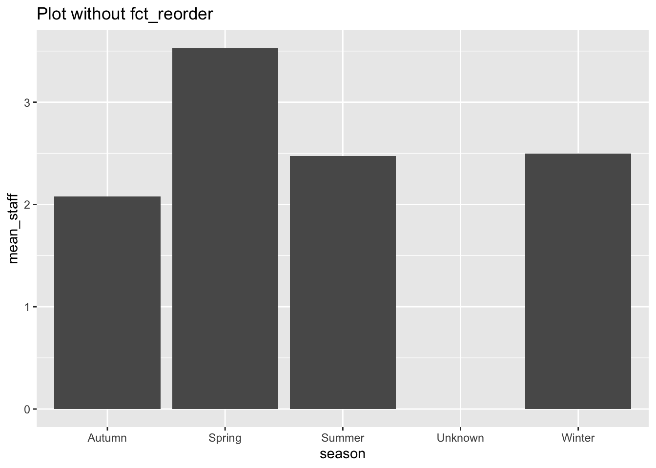


crew_group %>% 
  mutate(season = fct_reorder(season, desc(mean_staff))) %>% 
  ggplot(aes(x = season, y = mean_staff)) +
  geom_col() +
  labs(title = "Plot with fct_reorder")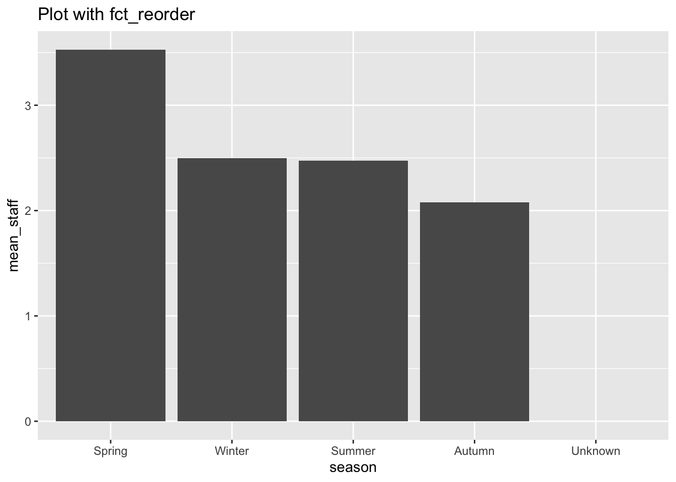


data_sorted <- crew_group %>% 
  mutate(season = fct_reorder(season, desc(mean_staff)))

levels(as.factor(crew_group$season))
#> [1] "Autumn"  "Spring"  "Summer"  "Unknown" "Winter"
levels(data_sorted$season)
#> [1] "Spring"  "Winter"  "Summer"  "Autumn"  "Unknown"

Once again we see that the order of levels has switched from alphabetical to a different order.

67.4.5 `fct_relevel`

This function is used to change the levels of a factor. When R deals with levels in a factor, it sorts the levels of the factor in alphabetical order. This means that if your factor includes temperatures like “hot,” “cold” and “medium,” R will make the levels “cold,” “hot,” “medium.” This can be tricky when classifying the factor because you may want it in increasing temperature or certain order.

fct_relevel takes three arguments: the factor you want to relevel, the new order of the levels and after which tells R where you want the new order to occur (you can set after=Inf to bring your order to the end.)

If you have a factor with levels “hot,” “cold” and “medium,” R will sort the levels alphabetically, meaning the order will be “cold,” “hot” and then “medium.” fct_relevel is one way to put the levels in the correct order. There are many ways to change the order, you can either write the order yourself or just move hot to the end using after = Inf.

temperatures <- factor(x = c("hot", "cold", "medium"))
levels(x = temperatures)
#> [1] "cold"   "hot"    "medium"

# use fct_relevel

fct_relevel(temperatures, "hot", after = Inf)
#> [1] hot    cold   medium
#> Levels: cold medium hot

Another example of using fct_relevel is with the expedition data. We can use it to change the levels of the termination_reason to place Successful expeditions at the top of the levels.

termination_levels <- levels(as.factor(expeditions$termination_reason))
reordered_levels <- fct_relevel(termination_levels, "Success (claimed)", "Success (main peak)",
            "Success (subpeak)")

levels(x = reordered_levels)
#>  [1] "Success (claimed)"                                                           
#>  [2] "Success (main peak)"                                                         
#>  [3] "Success (subpeak)"                                                           
#>  [4] "Accident (death or serious injury)"                                          
#>  [5] "Attempt rumoured"                                                            
#>  [6] "Bad conditions (deep snow, avalanching, falling ice, or rock)"               
#>  [7] "Bad weather (storms, high winds)"                                            
#>  [8] "Did not attempt climb"                                                       
#>  [9] "Did not reach base camp"                                                     
#> [10] "Illness, AMS, exhaustion, or frostbite"                                      
#> [11] "Lack (or loss) of supplies or equipment"                                     
#> [12] "Lack of time"                                                                
#> [13] "Other"                                                                       
#> [14] "Route technically too difficult, lack of experience, strength, or motivation"
#> [15] "Unknown"

Now we have successes at the top.

You can also include a function in fct_relevel to change up the order of your levels. You can use functions like sample, sort or rev to change the order.

termination_levels <- levels(as.factor(expeditions$termination_reason))
# use sample to make the order of levels randomized

levels(fct_relevel(termination_levels, sample))
#>  [1] "Illness, AMS, exhaustion, or frostbite"                                      
#>  [2] "Unknown"                                                                     
#>  [3] "Bad weather (storms, high winds)"                                            
#>  [4] "Success (claimed)"                                                           
#>  [5] "Success (subpeak)"                                                           
#>  [6] "Attempt rumoured"                                                            
#>  [7] "Accident (death or serious injury)"                                          
#>  [8] "Lack (or loss) of supplies or equipment"                                     
#>  [9] "Bad conditions (deep snow, avalanching, falling ice, or rock)"               
#> [10] "Lack of time"                                                                
#> [11] "Other"                                                                       
#> [12] "Success (main peak)"                                                         
#> [13] "Did not reach base camp"                                                     
#> [14] "Did not attempt climb"                                                       
#> [15] "Route technically too difficult, lack of experience, strength, or motivation"

67.5 Exercises

These next exercises will use a dataset which looks at the various countries who have given gifts to the United States, along with the monetary value of these gifts. While the original dataset has almost every country in the world, we will focus on a smaller portion of the countries.

#> Rows: 747
#> Columns: 10
#> $ id               <dbl> 3, 5, 6, 7, 13, 29, 51, 52, 57, 6…
#> $ recipient        <chr> "President", "President", "Presid…
#> $ agency_name      <chr> NA, NA, NA, NA, NA, NA, NA, NA, N…
#> $ year_received    <dbl> 1999, 1999, 1999, 1999, 1999, 199…
#> $ date_received    <date> NA, NA, NA, NA, NA, NA, NA, NA, …
#> $ donor            <chr> "Sr. Victor Cervera Pacheco, Gove…
#> $ donor_country    <chr> "Mexico", "Spain", "France", "Ita…
#> $ gift_description <chr> "49\" tall wood chair with a blac…
#> $ value_usd        <dbl> 1000, 660, 1200, 1400, 250, 800, …
#> $ justification    <chr> "Non-acceptance would cause embar…

Using fct_reorder change the order of the donor_country levels to be in order of mean_value.

gifts_grouped <- gifts %>% 
  group_by(donor_country) %>% 
  summarise(mean_value = mean(value_usd, na.rm = T))
## Enter solution below

gifts_grouped <- gifts %>% 
  group_by(donor_country) %>% 
  summarise(mean_value = mean(value_usd, na.rm = T))
## Enter solution below
fct_reorder(gifts_grouped$donor_country, gifts_grouped$mean_value)
#> [1] Australia Brazil    Canada    France    Germany  
#> [6] Italy     Mexico    Spain    
#> 8 Levels: Spain Canada Mexico Australia Germany ... Italy

Now, using fct_reorder change the order of the donor_country levels to be decreasing by mean_value. (Bonus: use the new order to make a plot, steps are very similar to the earlier examples)

gifts_grouped <- gifts %>% 
  group_by(donor_country) %>% 
  summarise(mean_value = mean(value_usd, na.rm = T))
## Enter solution below

gifts_grouped <- gifts %>% 
  group_by(donor_country) %>% 
  summarise(mean_value = mean(value_usd, na.rm = T))
## Enter solution below
fct_reorder(gifts_grouped$donor_country, desc(gifts_grouped$mean_value))
#> [1] Australia Brazil    Canada    France    Germany  
#> [6] Italy     Mexico    Spain    
#> 8 Levels: Italy Brazil France Germany Australia ... Spain

## BONUS
gifts_grouped %>% 
  mutate(donor_country = fct_reorder(donor_country, desc(mean_value))) %>% 
  ggplot(aes(donor_country, mean_value)) +
  geom_col()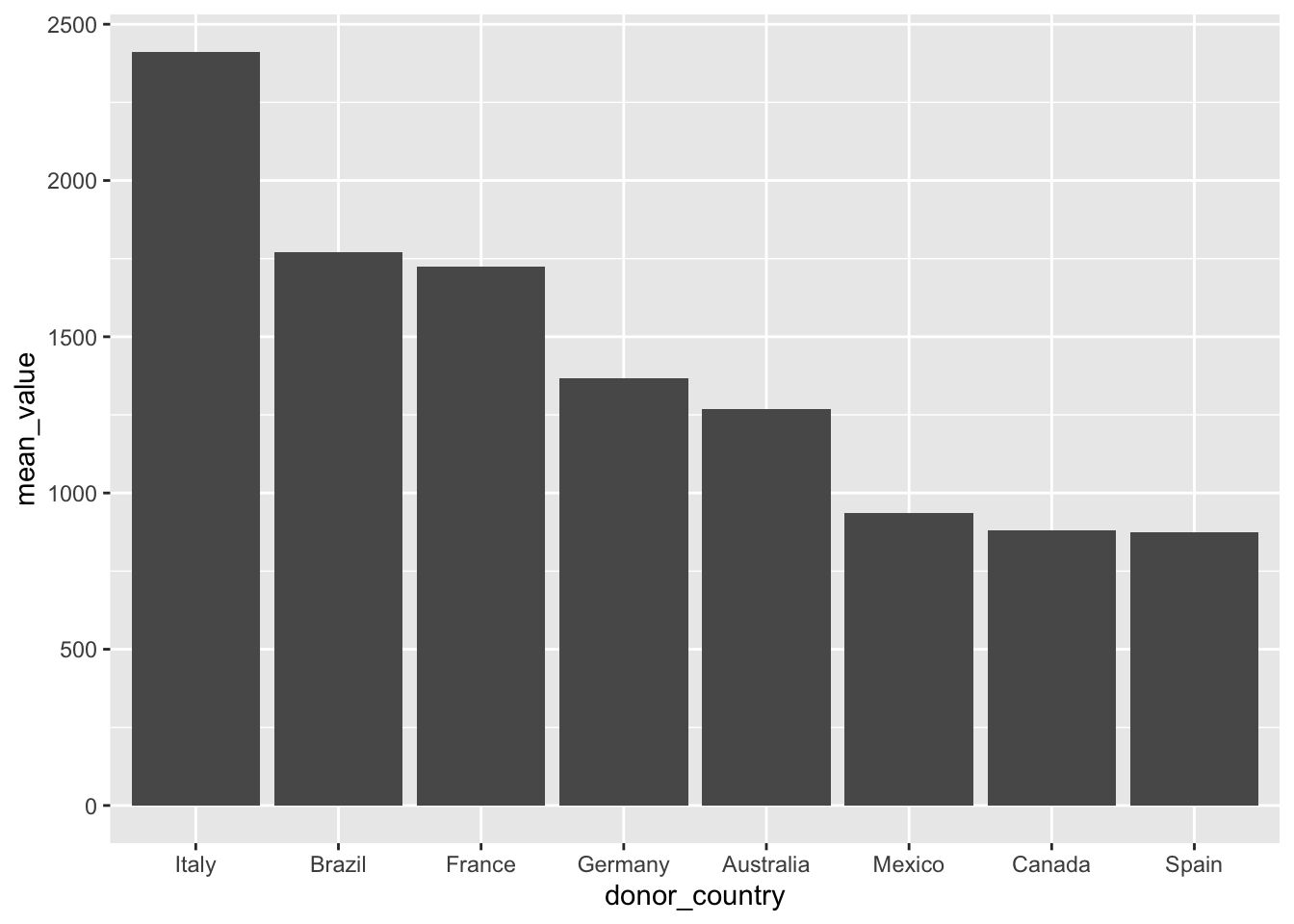

Using fct_relevel, change the order of the levels for gifts$donor_country to be randomly sampled.

fct_relevel(gifts$donor_country, sample)
#>   [1] Mexico    Spain     France    Italy     France   
#>   [6] Canada    Mexico    Mexico    Canada    France   
#>  [11] France    Germany   France    France    Italy    
#>  [16] Canada    Italy     Canada    Australia Australia
#>  [21] Mexico    Germany   Italy     Australia Australia
#>  [26] Spain     Italy     Italy     Italy     France   
#>  [31] Mexico    Mexico    Germany   Mexico    Italy    
#>  [36] France    Spain     Italy     Spain     Spain    
#>  [41] France    Mexico    Mexico    Australia Mexico   
#>  [46] Canada    Mexico    Mexico    Germany   Canada   
#>  [51] Canada    Mexico    Italy     Italy     Italy    
#>  [56] Italy     Italy     Italy     Italy     Italy    
#>  [61] Italy     Italy     Canada    Australia France   
#>  [66] Italy     France    Spain     Mexico    Canada   
#>  [71] Canada    Mexico    Canada    Spain     Spain    
#>  [76] Italy     Australia Australia Spain     Spain    
#>  [81] Italy     Italy     Italy     Italy     Mexico   
#>  [86] Italy     Mexico    Mexico    France    Italy    
#>  [91] Italy     Italy     Italy     France    Mexico   
#>  [96] Spain     Germany   Germany   France    Italy    
#> [101] Italy     Canada    Italy     Italy     Mexico   
#> [106] Germany   Italy     Mexico    Italy     Italy    
#> [111] Germany   Italy     France    Mexico    Italy    
#> [116] Australia Italy     Australia France    Italy    
#> [121] Spain     France    Brazil    Italy     Australia
#> [126] Italy     Italy     France    Australia Italy    
#> [131] Italy     Italy     Spain     Australia Australia
#> [136] Italy     France    Italy     Italy     Italy    
#> [141] Italy     Canada    Canada    Canada    Canada   
#> [146] Italy     Canada    Italy     Italy     France   
#> [151] France    Spain     Canada    Italy     Spain    
#> [156] Italy     France    Mexico    Canada    Spain    
#> [161] Mexico    Canada    Italy     Italy     Italy    
#> [166] Italy     Italy     Italy     Italy     France   
#> [171] Italy     Italy     Italy     Italy     Italy    
#> [176] Italy     Italy     France    Mexico    Mexico   
#> [181] Brazil    Canada    France    Italy     Italy    
#> [186] France    Italy     France    Germany   France   
#> [191] Canada    France    France    Canada    Mexico   
#> [196] Germany   Italy     France    Italy     Brazil   
#> [201] Brazil    Italy     Italy     Italy     Italy    
#> [206] Italy     Italy     France    Canada    Italy    
#> [211] Spain     Mexico    Mexico    Italy     Mexico   
#> [216] Italy     Germany   France    Italy     Canada   
#> [221] Germany   Italy     Italy     Australia Italy    
#> [226] Canada    Italy     Germany   Italy     Canada   
#> [231] Mexico    Germany   Australia Australia Canada   
#> [236] Germany   France    Germany   France    Mexico   
#> [241] Italy     Italy     Italy     Mexico    Germany  
#> [246] Germany   Germany   Germany   Italy     Germany  
#> [251] Italy     Australia Germany   Mexico    Mexico   
#> [256] Italy     Italy     France    France    France   
#> [261] Brazil    Australia France    France    France   
#> [266] Italy     Italy     Australia Australia Australia
#> [271] Australia Australia Australia Australia Australia
#> [276] Australia Australia Australia Australia Australia
#> [281] Australia Australia Australia Australia Australia
#> [286] Australia Australia Australia Australia Australia
#> [291] Australia Canada    Italy     Italy     Italy    
#> [296] Mexico    Mexico    Brazil    France    Mexico   
#> [301] Mexico    Mexico    Mexico    Mexico    Mexico   
#> [306] Italy     Italy     Italy     Australia Italy    
#> [311] France    Brazil    Italy     Italy     Italy    
#> [316] Italy     France    France    Australia Australia
#> [321] Australia France    France    France    France   
#> [326] France    Italy     Germany   Mexico    Mexico   
#> [331] France    France    France    France    Italy    
#> [336] Italy     Italy     Australia Germany   Mexico   
#> [341] France    Italy     Italy     France    Canada   
#> [346] Italy     Italy     Italy     Italy     Italy    
#> [351] Italy     Italy     Italy     France    Brazil   
#> [356] Brazil    Brazil    Brazil    Spain     Mexico   
#> [361] Mexico    Mexico    Brazil    Mexico    Mexico   
#> [366] Germany   France    France    Mexico    Italy    
#> [371] Spain     Italy     Mexico    Germany   Brazil   
#> [376] Germany   Germany   Italy     Italy     Mexico   
#> [381] Italy     Italy     France    Spain     France   
#> [386] Germany   Italy     Germany   France    France   
#> [391] Italy     France    Italy     Italy     Australia
#> [396] Italy     Italy     Italy     Italy     Italy    
#> [401] Italy     Italy     Italy     Brazil    Brazil   
#> [406] Germany   Spain     Germany   France    France   
#> [411] Germany   Spain     France    Canada    Canada   
#> [416] Canada    Canada    Germany   Germany   Germany  
#> [421] Australia Brazil    Germany   Canada    Brazil   
#> [426] Brazil    Germany   Brazil    France    France   
#> [431] Germany   Australia Mexico    France    France   
#> [436] France    Mexico    Brazil    France    Spain    
#> [441] France    Germany   France    Italy     Italy    
#> [446] Canada    Canada    Australia Canada    Australia
#> [451] Germany   France    Canada    Mexico    Australia
#> [456] Brazil    Brazil    Brazil    France    Germany  
#> [461] Italy     France    Australia Mexico    France   
#> [466] France    France    France    Mexico    France   
#> [471] Mexico    Brazil    France    Germany   France   
#> [476] Australia France    Brazil    Brazil    Brazil   
#> [481] Germany   Italy     Italy     Italy     Italy    
#> [486] Australia Brazil    Mexico    Mexico    Mexico   
#> [491] Mexico    Italy     Mexico    Mexico    Mexico   
#> [496] Spain     Spain     Italy     Italy     Italy    
#> [501] Mexico    Spain     Italy     Italy     France   
#> [506] Brazil    Canada    Germany   Italy     Canada   
#> [511] Italy     Italy     Italy     Italy     Italy    
#> [516] Canada    Canada    Mexico    Canada    Canada   
#> [521] Spain     Italy     Mexico    Spain     France   
#> [526] Canada    France    Mexico    Spain     Spain    
#> [531] France    Canada    Spain     Italy     Italy    
#> [536] Canada    Canada    Mexico    France    Germany  
#> [541] France    Brazil    Italy     France    Italy    
#> [546] Italy     Italy     Mexico    Mexico    Italy    
#> [551] Canada    Brazil    France    Australia Mexico   
#> [556] Mexico    Germany   Italy     Canada    Mexico   
#> [561] Australia Brazil    Mexico    Canada    Mexico   
#> [566] Mexico    Germany   Mexico    Italy     Spain    
#> [571] Australia Australia Italy     Germany   Germany  
#> [576] Italy     France    Italy     France    France   
#> [581] France    Canada    Italy     Italy     Germany  
#> [586] France    Mexico    Brazil    Mexico    Germany  
#> [591] Germany   Germany   Germany   Germany   Germany  
#> [596] Germany   Germany   Germany   Brazil    Brazil   
#> [601] France    Mexico    France    Mexico    Mexico   
#> [606] Italy     Australia Spain     France    Germany  
#> [611] France    Germany   Mexico    France    Italy    
#> [616] Australia France    Mexico    Italy     France   
#> [621] Australia France    Australia Italy     France   
#> [626] Mexico    Brazil    Spain     Mexico    France   
#> [631] France    Italy     Brazil    Canada    Australia
#> [636] Italy     Canada    France    Australia Canada   
#> [641] Canada    Spain     Germany   Italy     Italy    
#> [646] Mexico    Italy     Germany   Italy     Brazil   
#> [651] Germany   Mexico    Spain     Italy     Germany  
#> [656] Italy     France    Australia Canada    Canada   
#> [661] Italy     France    Spain     Italy     Canada   
#> [666] Italy     Mexico    Mexico    Australia France   
#> [671] Canada    Canada    Canada    France    Mexico   
#> [676] France    Brazil    France    Italy     Brazil   
#> [681] Mexico    Australia Australia Italy     Canada   
#> [686] Germany   Canada    Spain     Spain     Mexico   
#> [691] Italy     Germany   Canada    Canada    Italy    
#> [696] Spain     Brazil    Canada    Mexico    France   
#> [701] Mexico    Germany   Canada    Canada    Canada   
#> [706] Italy     Germany   Germany   France    Australia
#> [711] Italy     Germany   Germany   Canada    Germany  
#> [716] Germany   Germany   Germany   Germany   Germany  
#> [721] Germany   Germany   Germany   France    France   
#> [726] Germany   Mexico    Mexico    Mexico    Mexico   
#> [731] Mexico    France    Spain     Australia France   
#> [736] Canada    Italy     France    Australia France   
#> [741] Germany   Germany   Germany   Germany   Germany  
#> [746] Germany   Spain    
#> 8 Levels: Germany Spain Canada France Brazil ... Mexico

This final exercise will combine the uses of different forcats functions and will still use the gifts data. Using one of the fct_lump_ functions, lump all but 5 of the donor_country levels into other (save it under gifts_lumped). Next, using fct_relevel change the order to be in a random order (save under gifts_lumped again). Finally, using a forcats function count how many entries are in each level.

gifts_lumped <- fct_lump_n(gifts$donor_country, 5)
gifts_lumped <- fct_relevel(gifts_lumped, rev)
fct_count(gifts_lumped)
#> # A tibble: 6 × 2
#>   f             n
#>   <fct>     <int>
#> 1 Other       156
#> 2 Mexico      104
#> 3 Italy       199
#> 4 Germany      89
#> 5 France      125
#> 6 Australia    74

factor_example <- factor(c(rep("dog", 20), rep("cat", 19), 
                    rep("fish", 12), rep("cow", 9),
                    rep("bird", 24)))

fct_relevel(factor_example, "fish", "dog") 

fct_lump_n(factor_example, 2)

67.6 Common Mistakes & Errors

Error: "f" must be a factor (or character vector).
- This error will occur if you try to call forcats functions on non-factors. To fix this, ensure you are using a factor.
argument ".x" is missing, with no default
- This error will occur if you are missing an argument in your function call. Double check that you have filled out all arguments.

67.7 Next Steps

Now that you’re familiar with the forcats package, here are some additional resources to help continue your learning:

The forcats website which includes more examples and information about the most important functions: https://forcats.tidyverse.org/
R for Data Science’s chapter about factors. This chapter gives another lesson on factors and also uses the forcats package to work with factors: https://r4ds.had.co.nz/factors.html
The factors chapter from Jenny Bryan’s STAT 545 book: https://stat545.com/factors-boss.html

67.8 Questions

True or False, factors are stored as integer levels in R?

True
False

Which R package has tools to work with factors?

dplyr
forcast
forcats
ggplot2

Which function checks if a vector is a factor or not?

Which function counts the number of values in each level of your factor?

True or False, forcats functions can change how ggplot plots look?

True
False

Which function will allow me to change the order of my factors for a plot?

What is the cause of the "“f” must be a factor (or character vector)." error?

The function you are calling does not exist
The vector you are using does not exist
The vector you are using is not a factor
The function you are using is incorrect

Which function lumps levels that appear less than a certain proportion of times?

Which function takes factors with different levels and combines them into one factor?

True or False, forcats functions can be used with dplyr functions like mutate?

True
False

66 pull, pluck and unnest

68 More on strings