5 Hello World!
Written by Annie Collins and last updated on 7 October 2021.
5.1 Introduction
The purpose of this module is to give you an overview of a task you will be able to accomplish on your own once you gain some more experience using R. You do not need to understand the code; simply follow along and take note of any functions that seem interesting or useful to you!
In this scenario, let’s assume we’re working for Toronto Public Health and we’re looking at data about COVID-19 cases in Toronto throughout the pandemic. Specifically, we want to look at daily case numbers from different sources of infection - community spread, travel, outbreaks, etc. We have data collected by our front-line colleagues at the individual level, but it is slightly messy and contains more information than is relevant for our purposes.
First, we need to clean this data - make it as simple as possible and easy to work with - and then we can look into summarizing and examining different variables to draw conclusions about case numbers from different sources of infection.
5.2 Video walk through
This video provides a quick walkthrough of the process outlined in the following steps.
The following pages give a closer look at the individual functions and logic behind the loading, cleaning, and summarizing steps taken.
5.3 Load data
Before we can even access our data, we need to load our R libraries You will learn more about what this actually means later, but for now, think of loading libraries as us telling the computer which tools we need for our upcoming tasks.
Now we will load our data. Since our data is from Toronto Public Health, we are pulling it from the Toronto Open Data Portal and labeling it “covid_data.”
covid_data <-
  list_package_resources("https://open.toronto.ca/dataset/covid-19-cases-in-toronto/") %>%
  get_resource()
To get an initial idea of the variables (columns) we’re working with, we can load the first 20 rows of data and examine its contents and parameters. In R, this takes a form similar to a spreadsheet.
head(covid_data, 20)
#> # A tibble: 20 × 18
#>    `_id` Assigned_ID `Outbreak Associated` `Age Group`
#>    <dbl>       <dbl> <chr>                 <chr>
#>  1     1           1 Sporadic              50 to 59 Years
#>  2     2           2 Sporadic              50 to 59 Years
#>  3     3           3 Sporadic              20 to 29 Years
#>  4     4           4 Sporadic              60 to 69 Years
#>  5     5           5 Sporadic              60 to 69 Years
#>  6     6           6 Sporadic              50 to 59 Years
#>  7     7           7 Sporadic              80 to 89 Years
#>  8     8           8 Sporadic              60 to 69 Years
#>  9     9           9 Sporadic              50 to 59 Years
#> 10    10          10 Sporadic              60 to 69 Years
#> 11    11          11 Sporadic              70 to 79 Years
#> 12    12          12 Sporadic              50 to 59 Years
#> 13    13          13 Sporadic              60 to 69 Years
#> 14    14          14 Sporadic              30 to 39 Years
#> 15    15          15 Sporadic              40 to 49 Years
#> 16    16          16 Sporadic              50 to 59 Years
#> 17    17          17 Sporadic              20 to 29 Years
#> 18    18          18 Sporadic              40 to 49 Years
#> 19    19          19 Outbreak Associated   40 to 49 Years
#> 20    20         115 Sporadic              30 to 39 Years
#> # … with 14 more variables: `Neighbourhood Name` <chr>,
#> #   FSA <chr>, `Source of Infection` <chr>,
#> #   Classification <chr>, `Episode Date` <date>,
#> #   `Reported Date` <date>, `Client Gender` <chr>,
#> #   Outcome <chr>, `Currently Hospitalized` <chr>,
#> #   `Currently in ICU` <chr>, `Currently Intubated` <chr>,
#> #   `Ever Hospitalized` <chr>, `Ever in ICU` <chr>, …
Once all our data is loaded, we can start the cleaning process.
5.4 Clean existing data
The first step we will take is changing the “Episode Date” and “Reported Date” columns to a date format instead of a character format. This will allow us to use functions and operations with this data as if it were a date instead of as a string of characters.
covid_data$`Episode Date` <- as.Date(covid_data$`Episode Date`)
covid_data$`Reported Date` <- as.Date(covid_data$`Reported Date`)
Since we’re looking at source of infection, we don’t really care about the outcomes of individual cases. We also don’t need the “Outbreak Associated” column, since this data is contained (with more detail) in the “Source of Infection” column. To remove these unnecessary rows from our data, we can select only the rows we wish to keep.
covid_data <- select(covid_data, `Age Group`:Outcome)
unique(covid_data$`Source of Infection`)
#> [1] "Travel"                    "Healthcare"
#> [3] "N/A - Outbreak associated" "Close contact"
#> [5] "Community"                 "Unknown/Missing"
#> [7] "Institutional"             "Pending"
If we look at the classifications (unique values) for “Source of Infection,” we notice that “N/A - Outbreak associated” is a bit out of place given we have removed the “Outbreak Associated” column. We can replace this classification to more simply read “Outbreak associated.”
covid_data$`Source of Infection`[covid_data$`Source of Infection` == "N/A - Outbreak associated"] <- "Outbreak associated"Given the nature of this data, it is likely that the most recent date’s COVID-19 case data has not been recorded in its entirety and is inaccurate or an outlier to some extent, so we will also filter this data out of our data set.
head(covid_data, 20)
#> # A tibble: 20 × 9
#>    `Age Group`    `Neighbourhood Na…` FSA   `Source of Inf…`
#>    <chr>          <chr>               <chr> <chr>
#>  1 50 to 59 Years Willowdale East     M2N   Travel
#>  2 50 to 59 Years Willowdale East     M2N   Travel
#>  3 20 to 29 Years Parkwoods-Donalda   M3A   Travel
#>  4 60 to 69 Years Church-Yonge Corri… M4W   Travel
#>  5 60 to 69 Years Church-Yonge Corri… M4W   Travel
#>  6 50 to 59 Years Newtonbrook West    M2R   Travel
#>  7 80 to 89 Years Milliken            M1V   Travel
#>  8 60 to 69 Years Willowdale West     M2N   Travel
#>  9 50 to 59 Years Willowdale East     M2N   Travel
#> 10 60 to 69 Years Henry Farm          M2J   Travel
#> 11 70 to 79 Years Don Valley Village  M2J   Travel
#> 12 50 to 59 Years Lawrence Park South M4R   Travel
#> 13 60 to 69 Years Bridle Path-Sunnyb… M2L   Travel
#> 14 30 to 39 Years Moss Park           M5A   Healthcare
#> 15 40 to 49 Years Annex               M6G   Travel
#> 16 50 to 59 Years Willowdale East     M2N   Travel
#> 17 20 to 29 Years Westminster-Branson M2R   Travel
#> 18 40 to 49 Years Leaside-Bennington  M4G   Travel
#> 19 40 to 49 Years <NA>                <NA>  Outbreak associ…
#> 20 30 to 39 Years Moss Park           M5A   Travel
#> # … with 5 more variables: Classification <chr>,
#> #   `Episode Date` <date>, `Reported Date` <date>,
#> #   `Client Gender` <chr>, Outcome <chr>
Looking at our data as a whole, we can see that we’ve restricted the data to only the variables we want to work with, have reassigned the date columns to have type <date>, and have renamed an awkward variable classification in “Source of Infection.” Now we can summarize our data!
5.5 Summarize data
In our data, there are generally multiple cases reported per day, and we want to gain a better understanding of our variables across all cases reported on a given day. To do so, we will create a summary table from our original data listing the number of cases per source of infection, along with the total number of cases, for each day in our data.
covid_daily_stats <-
  covid_data %>%
  group_by(`Reported Date`) %>%
  summarise(
    travel = sum(`Source of Infection` == "Travel"),
    healthcare = sum(`Source of Infection` == "Healthcare"),
    outbreak = sum(`Source of Infection` == "Outbreak associated"),
    contact = sum(`Source of Infection` == "Close contact"),
    community = sum(`Source of Infection` == "Community"),
    unknown = sum(`Source of Infection` == "Unknown/Missing"),
    institutional = sum(`Source of Infection` == "Institutional"),
    pending = sum(`Source of Infection` == "Pending"),
    total = n()
    )
head(covid_daily_stats, 30)
#> # A tibble: 30 × 10
#>    `Reported Date` travel healthcare outbreak contact
#>    <date>           <int>      <int>    <int>   <int>
#>  1 2020-01-23           2          0        0       0
#>  2 2020-02-21           1          0        0       0
#>  3 2020-02-25           1          0        0       0
#>  4 2020-02-26           1          0        0       0
#>  5 2020-02-27           1          0        0       0
#>  6 2020-02-28           1          0        0       0
#>  7 2020-02-29           1          0        0       0
#>  8 2020-03-01           2          0        0       0
#>  9 2020-03-02           1          0        0       0
#> 10 2020-03-03           1          0        0       0
#> # … with 20 more rows, and 5 more variables:
#> #   community <int>, unknown <int>, institutional <int>,
#> #   pending <int>, total <int>
From this table, we can look at the daily summaries holistically or summarize further, for instance by looking at some summary statistics for daily COVID-19 case totals.
summary(covid_daily_stats$total)
#>    Min. 1st Qu.  Median    Mean 3rd Qu.    Max.
#>     1.0    45.0   154.0   247.5   380.0  1605.0
sum(covid_daily_stats$total)
#> [1] 83403
sum(covid_daily_stats$unknown)/sum(covid_daily_stats$total)
#> [1] 0.4224548
Now we know that the highest number of cases observed on a single day in the pandemic thus far is 1605, and that at least half of the recorded dates have seen over 154 cases. We can also see from the second and third calculations that there have been 83,403 in Toronto in total since the beginning of the pandemic, and that cases of unknown origin make up just over 42 percent of all cases. If we wanted to, we could go on to create graphs from this summary, like total cases per day over time or number of cases per source of infection.
colors <- c("Outbreak associated" = "red", "Close contact" = "blue", "Community spread" = "purple")
covid_daily_stats %>%
  ggplot(aes(x=`Reported Date`)) +
  geom_line(aes(y=outbreak, color = "Outbreak associated"), group=1) +
  geom_line(aes(y=contact, color = "Close contact"), group=1) +
  geom_line(aes(y=community, color = "Community spread"), group=1) +
  labs(x="Reported Date", y="Number of Cases", color="Source of Infection") +
  ggtitle("COVID-19 Cases in Toronto") +
  scale_color_manual(values = colors)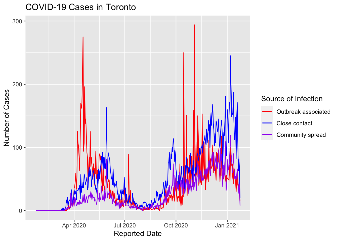
5.6 Next steps
This may all seem very complex and unattainable right now, but when it’s broken-down step by step (or function by function) it will gradually become easier to see how you can use R to produce your desired statistics, graphics, and analyses.
As you proceed through the following lessons, remember the process outlined here and take note of how powerful simple, individual functions can be when used together in the right context. You may also find it helpful to refer to this module as an example of different functions used in context, or to see if you can use your new knowledge to reproduce the same results on your own. Good luck!