7 Hello World, yet again!

Written by Simone Collier and last updated on 7 October 2021.

7.1 Introduction

In this module we will do a brief overview of R Markdown and run through an example of when it would be useful. R Markdown is a tool for creating reproducible reports that are formatted for the purpose of sharing with others. R Markdown effectively allows you to insert chunks of code with the option of several languages and execute them inside a document outputted as a PDF, HTML, or Word file. This function is particularly useful when you want to include your code, your results, and an explanation of both that goes beyond basic comments.

Suppose you have an assignment for a course that asks you to analyze, visualize, and interpret data about COVID vaccines. This would be the perfect opportunity to use R Markdown.

7.2 Doing the assignment in an R Script

To start off, let’s try to do this assignment in a normal R script. We start by importing the libraries we plan on using.

library(utils)
library(tidyverse)
library(knitr)

Now we can go ahead and import our data from Ontario’s data catalogue and look at the data set.

hospital_data <-
  read.csv(
    "https://data.ontario.ca/dataset/752ce2b7-c15a-4965-a3dc-397bf405e7cc/resource/274b819c-5d69-4539-a4db-f2950794138c/download/vac_status_hosp_icu.csv"
  )

head(hospital_data)
#>         date icu_unvac icu_partial_vac icu_full_vac
#> 1 2021-08-10        22               3            0
#> 2 2021-08-11        37               5            2
#> 3 2021-08-12        45               5            2
#> 4 2021-08-13        52               5            3
#> 5 2021-08-14        53               4            1
#> 6 2021-08-15        44               6            1
#>   hospitalnonicu_unvac hospitalnonicu_partial_vac
#> 1                   23                          4
#> 2                   34                          7
#> 3                   44                          7
#> 4                   65                          6
#> 5                   67                          6
#> 6                   58                          4
#>   hospitalnonicu_full_vac
#> 1                      11
#> 2                       8
#> 3                       9
#> 4                       8
#> 5                      11
#> 6                      14

We decide to look at patients in the ICU and their corresponding vaccine status. So, we choose the first four columns and ignore the rest.

icu_data <- hospital_data[, 1:4]
head(icu_data)
#>         date icu_unvac icu_partial_vac icu_full_vac
#> 1 2021-08-10        22               3            0
#> 2 2021-08-11        37               5            2
#> 3 2021-08-12        45               5            2
#> 4 2021-08-13        52               5            3
#> 5 2021-08-14        53               4            1
#> 6 2021-08-15        44               6            1

We plan to look at the proportions of the people in ICU that are in each category of vaccine status. Let’s take the daily mean number of patients in ICU and find the percentage in each category.

icu_means <- colMeans(hospital_data[, 2:4])
icu <- data.frame(
  'Vaccine_Status' = names(icu_means),
  'Mean_Daily_Patients' = unname(icu_means)
)
icu$Percentage_of_Means <- round((icu$Mean_Daily_Patients /
                                    sum(icu$Mean_Daily_Patients)) * 100, 1)

Now that we have some results let’s go ahead and make a visualization of this data in order to communicate these results. We can make a pie chart using the ggplot2 package.

# Compute the position of pie chart labels
icu <- icu %>%
  mutate(ypos = cumsum(Percentage_of_Means) - 0.5 * Percentage_of_Means)

ggplot(icu, aes(x = "", y = Percentage_of_Means, fill = Vaccine_Status)) +
  geom_bar(stat = "identity", width = 1) +
  coord_polar("y", start = 0) +
  theme_void() +
  geom_text(aes(y = ypos, label = paste(sprintf(
    "%.1f", round(Percentage_of_Means, 1)
  ),
  '%', sep = '')),
  color = "white", size = 4) +
  scale_fill_brewer(palette = "Set1")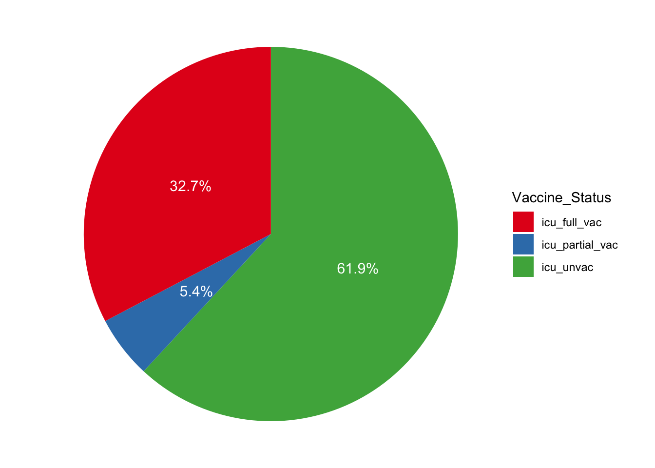

Great! We have finished the coding part of our assignment. Let’s look at our R Script that we wrote our assignment in.

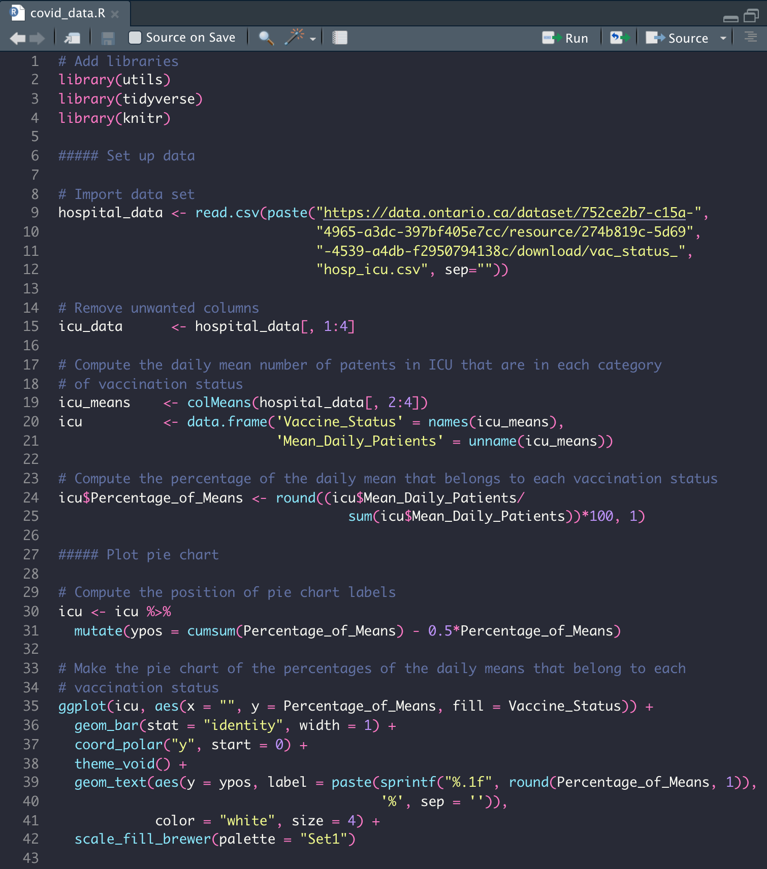
As we can see, this document only provides the code that we used to get our results along with some brief comments. If we submitted this document alone our prof would not be impressed since we haven’t shown any of the data that we’re using, the visualization that we worked to produce, or made any comments on our results. This is where R Markdown comes in to allow the integration of all these moving parts.

7.3 Doing the assignment in R Markdown

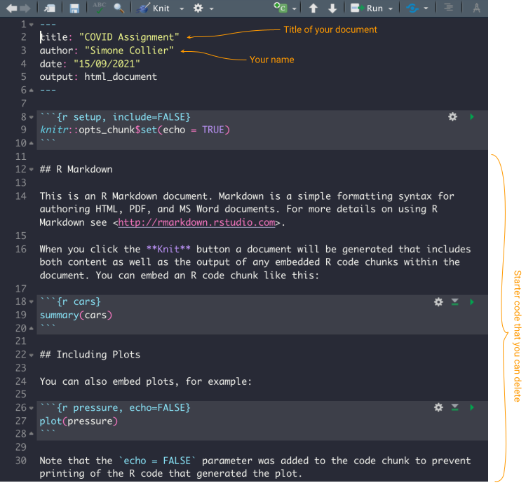
To start off let’s make a new R Markdown file and choose our output to be html. This opens an untitled file with example code.

We will use the same code we used in the R Script to get our results. So, in the first code chunk we can include all the libraries we plan on using.

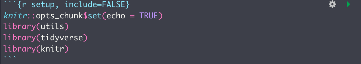
Note that this chunk of code will not be included in the outputted document due to include = FALSE (we can delete this if we want the chunk included). The next thing we did was import the data from Ontario’s data catalogue. We can execute code inline by typing `r CODE GOES HERE `, or with a new code chunk by typing

```{r}

CODE GOES HERE

```

We can also click in the bar above the script to add a code chunk. In our R Script, we used the function head() to see the first few rows of our data sets. The output is poorly formatted and can be annoying to read. Instead, we can use kable() (from the knitr package) which is specifically for outputting beautiful tables in R Markdown.

hospital_data <-
  read.csv(
    "https://data.ontario.ca/dataset/752ce2b7-c15a-4965-a3dc-397bf405e7cc/resource/274b819c-5d69-4539-a4db-f2950794138c/download/vac_status_hosp_icu.csv"
  )
icu_data      <- hospital_data[, 1:4]
icu_data$date <- as.Date(hospital_data$date)
kable(head(icu_data), format = 'simple')

date	icu_unvac	icu_partial_vac	icu_full_vac
2021-08-10	22	3	0
2021-08-11	37	5	2
2021-08-12	45	5	2
2021-08-13	52	5	3
2021-08-14	53	4	1
2021-08-15	44	6	1

7.4 The assignment

While we add the code from our R Script into our R Markdown file in code chunks, we can also write explanations of our methods and results outside of the chunks. After this, we end up with a beautiful R Markdown file that looks like this:

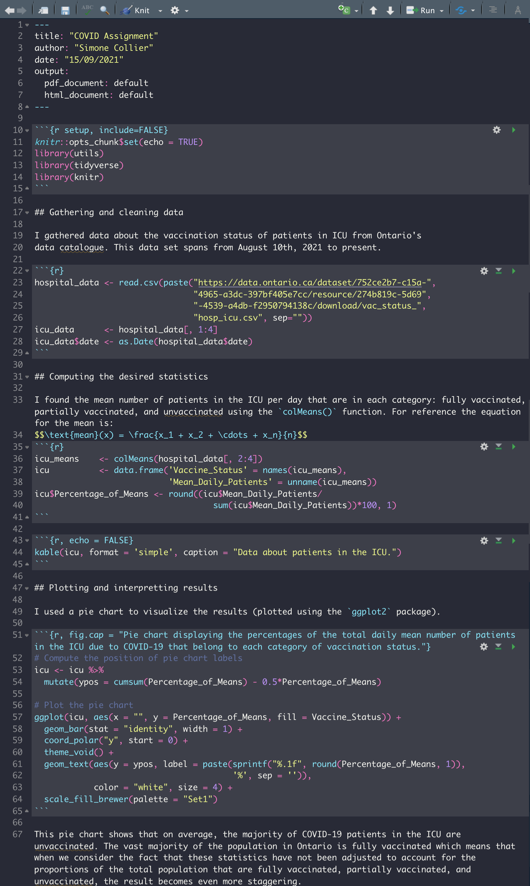
Don’t worry about understanding all the code that was included, the purpose of this example is to show how we might use R Markdown and the different features it offers.

We click on the on the arrow beside the “Knit” button

in the bar above the script, and we choose “Knit to PDF.” (Note that we can knit the document as many times as we like as we are writing. Every time we knit the document, the previous knitted file is replaced with the new version.)

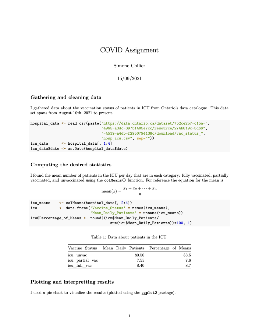
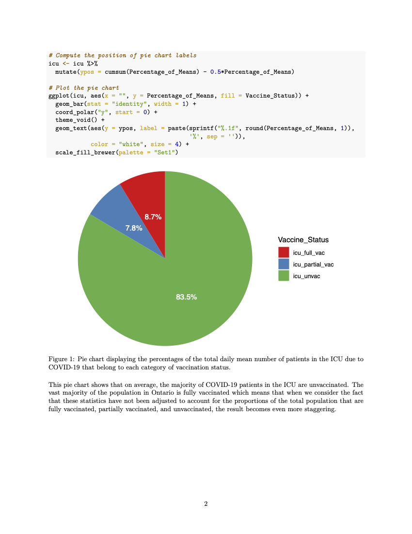
Our outputted file is easy to read, includes the chunks of code that are relevant to our analysis and omits those that aren’t using {r, include = FALSE} or {r, echo = FALSE}. We can create tables and plots just as we are in a normal R script, and we have the option to include captions to go alongside them. R Markdown allows us to write in \(LaTeX\) so that equations (such as the mean in our case) and symbols can be added seamlessly. We now have PDF file that is well formatted and ready to share.

While knitting to a PDF or Word are both great for the purpose of assignments, we also have the option to output in HTML which we can launch in a browser. This is great for making blog posts and showcasing your work in that manner. To get an idea of what that might look like, all the DoSS Toolkit modules are written in R Markdown and outputted as a form of HTML, so you are currently reading an R Markdown output! Beautiful, isn’t it?

As we can see, R Markdown is a great tool for integrating code and language to effectively communicate your results. See the DoSS Toolkit R Marky Markdown section for an in-depth lesson in R Markdown.

6 Hello World, again!

8 The R community