28 The pipe
Written by Mariam Walaa and last updated on 7 October 2021.
28.1 Introduction
In this lesson, you will learn how to:
- Load the package required to use the pipe
%>% - Use the pipe
%>%
Prerequisite skills include:
- Loading packages
Highlights:
- The pipe
%>%is used to keep code clean and concise. - The pipe
%>%works by piping data into a function. - The pipe
%>%can pipe data into functions repeatedly.
28.2 Overview
The pipe is helpful for keeping your code clean when you have to apply multiple
transformations to your data. You can start using the pipe after you have loaded the
magrittr package. The magrittr package is also part of tidyverse, so if you have
already loaded tidyverse then you will be able to start using the pipe.
In this tutorial, we will be using the penguins data to present the uses of the pipe. This
data contains records on measurements for penguin species, including their size, sex, and
where they live. There are 344 rows and 8 columns in this data set.

Figure: The Palmer Penguins Credits: Allison Horst
Lets start with loading the tidyverse.
Here is an example using base R summary() function, without using the pipe.
summary(penguins)
#>       species          island    bill_length_mm
#>  Adelie   :152   Biscoe   :168   Min.   :32.10
#>  Chinstrap: 68   Dream    :124   1st Qu.:39.23
#>  Gentoo   :124   Torgersen: 52   Median :44.45
#>                                  Mean   :43.92
#>                                  3rd Qu.:48.50
#>                                  Max.   :59.60
#>                                  NA's   :2
#>  bill_depth_mm   flipper_length_mm  body_mass_g
#>  Min.   :13.10   Min.   :172.0     Min.   :2700
#>  1st Qu.:15.60   1st Qu.:190.0     1st Qu.:3550
#>  Median :17.30   Median :197.0     Median :4050
#>  Mean   :17.15   Mean   :200.9     Mean   :4202
#>  3rd Qu.:18.70   3rd Qu.:213.0     3rd Qu.:4750
#>  Max.   :21.50   Max.   :231.0     Max.   :6300
#>  NA's   :2       NA's   :2         NA's   :2
#>      sex           year
#>  female:165   Min.   :2007
#>  male  :168   1st Qu.:2007
#>  NA's  : 11   Median :2008
#>               Mean   :2008
#>               3rd Qu.:2009
#>               Max.   :2009
#>
Here is code providing the same output using the pipe.
penguins %>% summary()
#>       species          island    bill_length_mm
#>  Adelie   :152   Biscoe   :168   Min.   :32.10
#>  Chinstrap: 68   Dream    :124   1st Qu.:39.23
#>  Gentoo   :124   Torgersen: 52   Median :44.45
#>                                  Mean   :43.92
#>                                  3rd Qu.:48.50
#>                                  Max.   :59.60
#>                                  NA's   :2
#>  bill_depth_mm   flipper_length_mm  body_mass_g
#>  Min.   :13.10   Min.   :172.0     Min.   :2700
#>  1st Qu.:15.60   1st Qu.:190.0     1st Qu.:3550
#>  Median :17.30   Median :197.0     Median :4050
#>  Mean   :17.15   Mean   :200.9     Mean   :4202
#>  3rd Qu.:18.70   3rd Qu.:213.0     3rd Qu.:4750
#>  Max.   :21.50   Max.   :231.0     Max.   :6300
#>  NA's   :2       NA's   :2         NA's   :2
#>      sex           year
#>  female:165   Min.   :2007
#>  male  :168   1st Qu.:2007
#>  NA's  : 11   Median :2008
#>               Mean   :2008
#>               3rd Qu.:2009
#>               Max.   :2009
#>
As you can see, the pipe %>% operator takes the penguins data frame and pipes it into
the summary() function, so you do not need to pass penguins as a parameter to
summary().
In this example, it is hard to see why using the pipe makes the code clean and concise, but when you have multiple transformations that you want to apply to your data, it becomes clearer why using the pipe makes your code cleaner, more concise, and easier to read.
Here is a similar example without the pipe, but this time we will also filter the data before we summarize it using the summary function.
adelie <- filter(penguins, species == "Adelie")
summary(adelie)
#>       species          island   bill_length_mm
#>  Adelie   :152   Biscoe   :44   Min.   :32.10
#>  Chinstrap:  0   Dream    :56   1st Qu.:36.75
#>  Gentoo   :  0   Torgersen:52   Median :38.80
#>                                 Mean   :38.79
#>                                 3rd Qu.:40.75
#>                                 Max.   :46.00
#>                                 NA's   :1
#>  bill_depth_mm   flipper_length_mm  body_mass_g
#>  Min.   :15.50   Min.   :172       Min.   :2850
#>  1st Qu.:17.50   1st Qu.:186       1st Qu.:3350
#>  Median :18.40   Median :190       Median :3700
#>  Mean   :18.35   Mean   :190       Mean   :3701
#>  3rd Qu.:19.00   3rd Qu.:195       3rd Qu.:4000
#>  Max.   :21.50   Max.   :210       Max.   :4775
#>  NA's   :1       NA's   :1         NA's   :1
#>      sex          year
#>  female:73   Min.   :2007
#>  male  :73   1st Qu.:2007
#>  NA's  : 6   Median :2008
#>              Mean   :2008
#>              3rd Qu.:2009
#>              Max.   :2009
#>
Equivalently, here is code providing the same output, using the pipe instead.
penguins %>%
  filter(species == "Adelie") %>%
  summary()
#>       species          island   bill_length_mm
#>  Adelie   :152   Biscoe   :44   Min.   :32.10
#>  Chinstrap:  0   Dream    :56   1st Qu.:36.75
#>  Gentoo   :  0   Torgersen:52   Median :38.80
#>                                 Mean   :38.79
#>                                 3rd Qu.:40.75
#>                                 Max.   :46.00
#>                                 NA's   :1
#>  bill_depth_mm   flipper_length_mm  body_mass_g
#>  Min.   :15.50   Min.   :172       Min.   :2850
#>  1st Qu.:17.50   1st Qu.:186       1st Qu.:3350
#>  Median :18.40   Median :190       Median :3700
#>  Mean   :18.35   Mean   :190       Mean   :3701
#>  3rd Qu.:19.00   3rd Qu.:195       3rd Qu.:4000
#>  Max.   :21.50   Max.   :210       Max.   :4775
#>  NA's   :1       NA's   :1         NA's   :1
#>      sex          year
#>  female:73   Min.   :2007
#>  male  :73   1st Qu.:2007
#>  NA's  : 6   Median :2008
#>              Mean   :2008
#>              3rd Qu.:2009
#>              Max.   :2009
#>
The code looks a lot cleaner, and we did not have to separate the process into two different steps or assign the filtered data to an object.
28.3 Exercises
You can learn more about the penguin characteristics and what they describe through this illustration by Allison Horst.
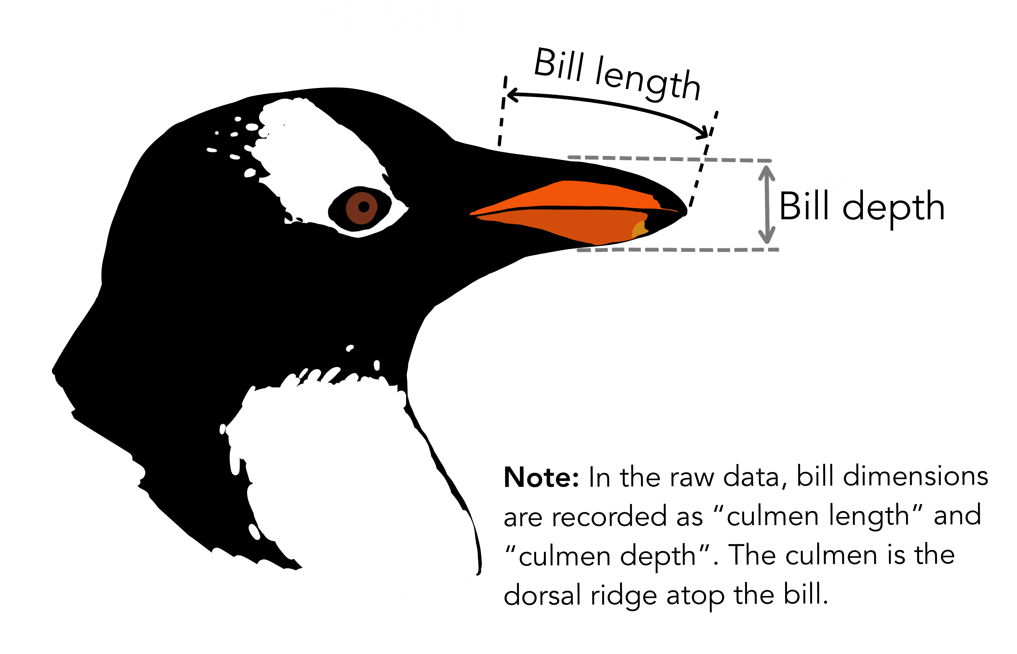
Figure: The Palmer Penguins Credits: Allison Horst
28.3.1 Exercise 1
Here is some code that filters the data first by species and then by sex, and summarizes the data using the summary function from above.
adelie <- filter(penguins, species == "Adelie")
female_adelie <- filter(adelie, sex == "female")
summary(female_adelie)
#>       species         island   bill_length_mm
#>  Adelie   :73   Biscoe   :22   Min.   :32.10
#>  Chinstrap: 0   Dream    :27   1st Qu.:35.90
#>  Gentoo   : 0   Torgersen:24   Median :37.00
#>                                Mean   :37.26
#>                                3rd Qu.:38.80
#>                                Max.   :42.20
#>  bill_depth_mm   flipper_length_mm  body_mass_g
#>  Min.   :15.50   Min.   :172.0     Min.   :2850
#>  1st Qu.:17.00   1st Qu.:185.0     1st Qu.:3175
#>  Median :17.60   Median :188.0     Median :3400
#>  Mean   :17.62   Mean   :187.8     Mean   :3369
#>  3rd Qu.:18.30   3rd Qu.:191.0     3rd Qu.:3550
#>  Max.   :20.70   Max.   :202.0     Max.   :3900
#>      sex          year
#>  female:73   Min.   :2007
#>  male  : 0   1st Qu.:2007
#>              Median :2008
#>              Mean   :2008
#>              3rd Qu.:2009
#>              Max.   :2009
As an exercise, try to convert the code above into equivalent code using the pipe.
# You don't have to assign it to an object
# You can filter multiple times within filter()28.3.2 Exercise 2
Here is some code that filters the data, first by sex and then by year of study, and counts the number of penguins using the count function.
females <- filter(penguins, sex == "female")
females_2007 <- filter(females, year == "2007")
count(females_2007)
#> # A tibble: 1 × 1
#>       n
#>   <int>
#> 1    51
As another exericse, try to convert the code above into equivalent code using the pipe.
# You don't have to assign it to an object28.4 Common Mistakes & Errors
Below are some common mistakes and errors you may come across:
- You might type the wrong operator. The pipe operator is as follows:
%>% - You might try to pipe something into a function other than data.