105 Static maps using ggmap
Written by Annie Collins and last updated on 7 October 2021.
105.1 Introduction
ggmapis an R package that makes it easy to retrieve raster map tiles from popular online mapping services like Google Maps and Stamen Maps and plot them using the ggplot2 framework
Now that you’re familiar with ggplot2 and its plotting capabilities, we can start looking at some more advanced data visualization options. Next up: maps.
In this lesson, you will learn how to:
- Use
ggmapto plot geospatial data over maps; and - Access Google Maps APIs to extend
ggmap’s functions to Google Maps as well.
Prerequisite skills include:
- Familiarity with
ggplot2and its plotting functions, specificallygeom_point()andstat_density2d().
105.2 Package
Unless you have worked with ggmap before, you will likely have to install the package from GitHub (it is also available from CRAN, but GitHub contains the most up-to-date version which is important in this case given that the package works with external APIs).
devtools::install_github("dkahle/ggmap")
library(ggmap)
105.3 Backgrounds
Much like the way you build a plot in ggplot2, ggmap plots are constructed by adding to your plot feature by feature, starting with a map background. ggmap allows you to use map backgrounds from two different sources: Google Maps and Stamen. Both offer several options for aesthetics and customization and are fairly similar in their use. Google Maps requires access to Google APIs (see Section 105.5 below) while Stamen Maps authentication is built into the package, so we will focus on Stamen backgrounds for the purpose of this lesson.
For a Stamen Map background, we use the function get_stamenmap(). This function takes several arguments that allow you to customize the appearance and format of your map, but most importantly you must state the boundaries, scale, and type of your map. The object produced by get_stamenmap() then gets passed to the ggmap() function which allows you to view the map in the “Plots” tab as well as display data on top of it.
| Argument | Parameter | Details |
|---|---|---|
| bbox | vector | A vector stating the locations of the corners of your desired map in the format c(lower left longitude, lower left latitude, upper right longitude, upper right latitude) |
| zoom | numeric | Level of zoom into focus area |
| maptype | string | Aesthetic of map produced. Options are: “terrain,” “terrain-background,” “terrain-labels,” “terrain-lines,” “toner,” “toner-2010,” “toner-2011,” “toner-background,” “toner-hybrid,” “toner-labels,” “toner-lines,” “toner-lite,” and “watercolor.” |
See ?get_stamenmap for additional arguments and details.
# Houston, Texas
map <- get_stamenmap(c(-95.39681, 29.73631, -95.34188, 29.78400), zoom = 15, maptype = "toner")

ggmap(map)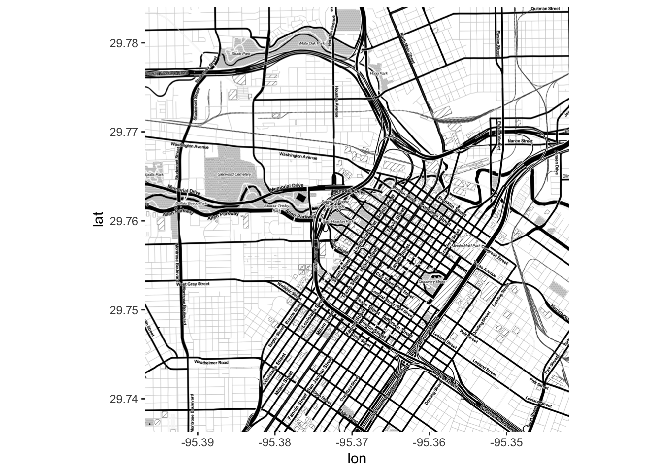
Tip: If you don’t know the exact coordinates of the map you wish to use as a background, clicking anywhere on Google Maps will give you the longitude and latitude of the selected location.
One thing that is important to know is that when loading map backgrounds we are working with longitude and latitude coordinates in decimal degree format. It is important to take note of the relative values of coordinates when defining map boundaries, and these will change depending on which hemisphere you’re in. In North America (the northern and western hemispheres), the lower left hand corner of the map will always be the smaller longitude value (farthest west) and the smaller latitude value (farthest south). The image below might help you to visualize the relationship between coordinate values.
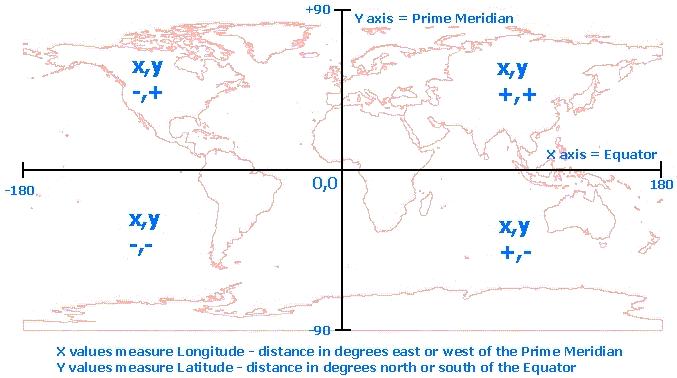
Figure 105.1: Source: Esri
105.4 Plotting Data
Now we can start to visualize some data on top using our familiar ggplot2 functions. We will be using the data set crime that is built into the ggmap package. Any data used with ggmap must have variables for longitude and latitude coordinates in decimal degree format for each observation, as these serve as the x and y coordinates when graphing on top of a map background.
A useful way to visualize data in this context is a scatterplot using geom_point().
# Filter out data points that fall outside of our mapped area, and thefts (which we will look at separately later)
local_crime <- ggmap::crime %>% filter(-95.39681 <= lon & lon <= -95.34188, 29.73631 <= lat & lat <=  29.78400, offense != "theft")

map <- get_stamenmap(c(-95.39681, 29.73631, -95.34188, 29.78400), zoom = 15, maptype = "toner")

ggmap(map) + geom_point(data = local_crime, aes(x=lon, y=lat, colour = offense)) +
  ggtitle("Crimes Reported in Houston, Texas, 2010") +
  xlab("Longitude") +
  ylab("Latitude")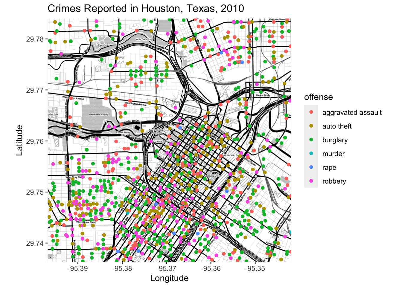
For crimes that appear very frequently in the data set, it might be more useful to use a heat map to track density instead of individual reports. We can see what this looks like using the thefts from the crime data set.
# Filter out data points that fall outside of our mapped area, and all offenses except theft
local_theft <- crime %>% filter(-95.39681 <= lon & lon <= -95.34188, 29.73631 <= lat & lat <=  29.78400, offense == "theft")

ggmap(map) + stat_density2d(data = local_theft, aes(x=lon, y=lat, fill = ..level.., alpha = 0.5), geom = "polygon") +
  scale_fill_gradient2(name = "Thefts") +
  ggtitle("Density of Thefts Reported in Houston, Texas, 2010") +
  xlab("Longitude") +
  ylab("Latitude")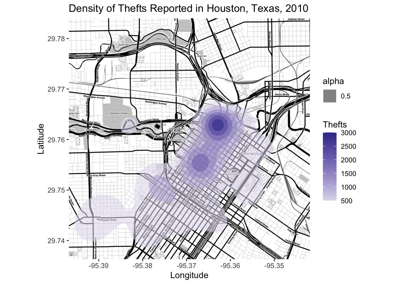
Like ggplot2, ggmap also works with facet_wrap(). Suppose we want to compare aggravated assaults and auto theft in Houston.
assault_auto <- crime %>% filter(-95.39681 <= lon & lon <= -95.34188, 29.73631 <= lat & lat <=  29.78400, offense == "aggravated assault" | offense == "auto theft")

ggmap(map) + stat_density2d(data = assault_auto, aes(x=lon, y=lat, fill = ..level.., alpha = 0.4), geom = "polygon") +
  scale_fill_gradient2(name = "Reports") +
  ggtitle("Density of Crimes Reported in Houston, Texas, 2010") +
  xlab("Longitude") +
  ylab("Latitude") +
  facet_wrap(~ offense)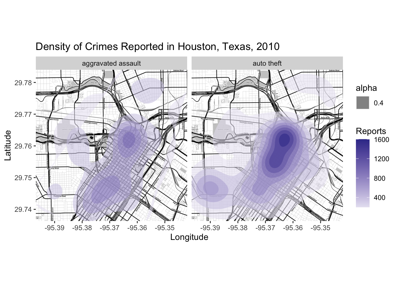
105.5 Google Maps APIs
In addition to Stamen Maps, ggmap can draw on Google Maps APIs for its Google Maps backgrounds, and in order to do this you must first register with Google. This involves creating an account if you do not already have a Google account, as well as registering a valid credit card (it will not be charged unless you select an account upgrade that requires payment).
To begin, go to the Google Maps Platform website. Follow the instructions to register an account and a payment method (credit card), and you will receive an API key. This is important! You need to register this within R and RStudio using the following code:

register_google(key = "[your key]", write = TRUE) # Copy and paste your API key in quotationsYou also want to make sure that you don’t share this key with anyone since it is private and personal to each user, so keep this in mind if you’re sharing your code anywhere.
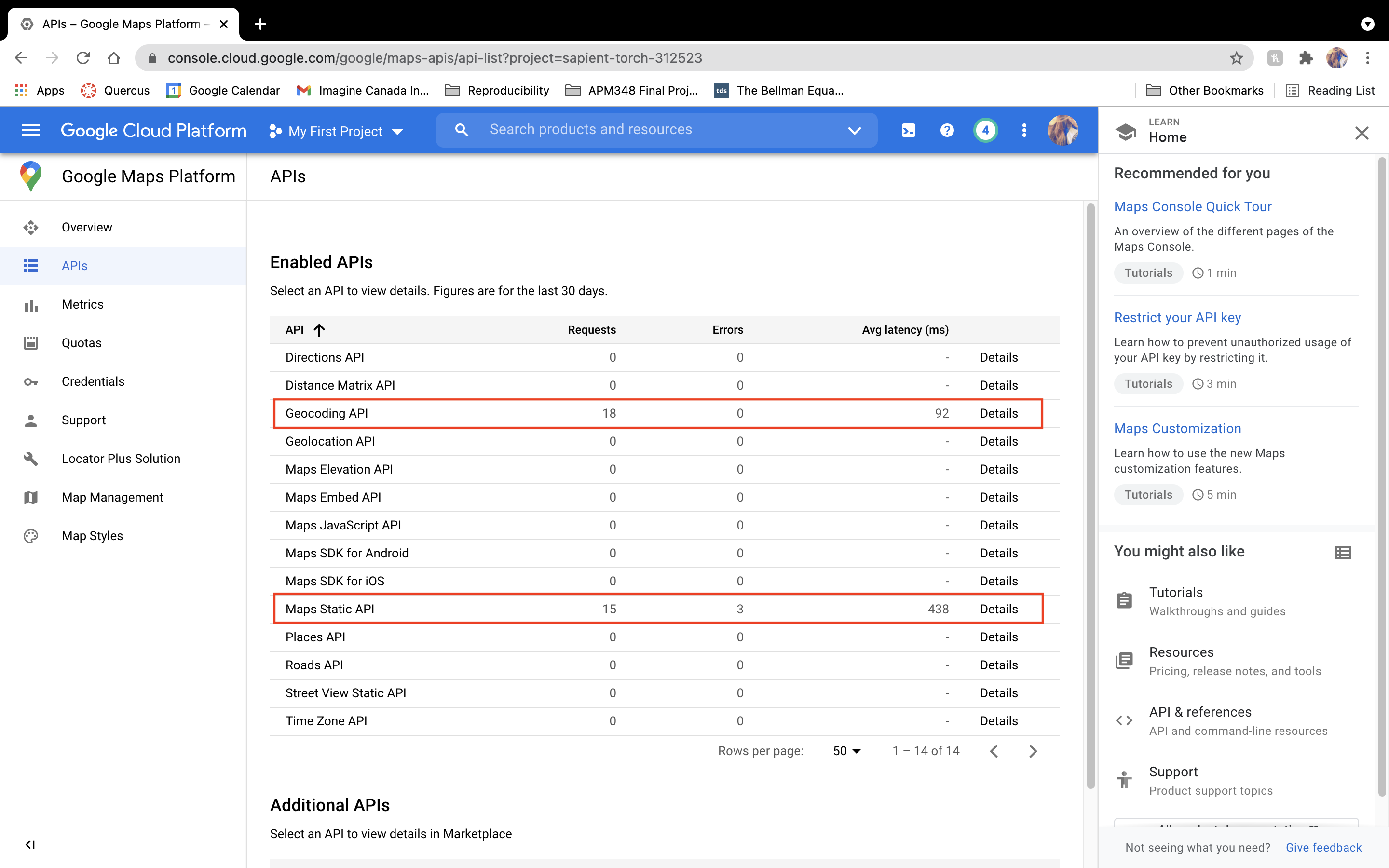
Once you’ve gained access to the Google Maps Platform you will need to enable the relevant APIs: Geocoding and Maps Static. These are the APIs that work with the functions in ggmap, specifically get_googlemap() (analogous to get_stamenmap()), geocode(), and revgeocode(). These functions cannot be demonstrated within this module until you have access to the appropriate APIs, but the ggmap repository README contains some examples and resources for using Google Maps with ggmap.

105.6 Next Steps
- Once you have the Google Maps APIs working on your system, repeat the above exercises using
get_googlemap()in place ofget_stamenmap(); - Use
ggimageto create more complex icon maps (check out this tutorial from R user and data scientist Laura Ellis); - Check out the
usmapspackage for more mapping functions specific to the United States.
105.7 Exercises
105.7.1 Question 1
For North American maps, which corner of the map boundary will be indicated by the smallest latitude coordinate and the smallest longitude coordinate?
- Upper left
- Upper right
- Lower left
- Lower right
105.7.2 Question 2
In the get_stamenmap() function argument bbox, what order do the coordinates appear in the vector?
- Lower left longitude, lower left latitude, upper right longitude, upper right latitude
- Lower left latitude, lower left longitude, upper right latitude, upper right longitude
- Upper right longitude, upper right latitude, lower left longitude, lower left latitude
- Upper right latitude, upper right longitude, lower left latitude, lower left longitude
105.7.3 Question 3
Consider a data set called covid_testing_locations. Suppose variable LocationType has three distinct categories and variable TestType has two distinct categories. Which of the following correctly describes the output of toronto_map %>% ggmap() + geom_point(data=covid_testing_locations, aes(x=lat, y=long)) + facet_wrap(~LocationType)
- One map with two legends, one for
LocationTypeand one forTestType. - Two of the same map object, each displaying locations for a specific test category from
TestType. - Two of the same map object, each displaying locations for a specific location category from
LocationType. - Six of the same map object, each displaying locations for a unique combination of
LocationTypeandTestType.
105.7.4 Question 4
If toronto_map refers to the output of get_stamenmap() with coordinates inputted for Toronto, which of the following will correctly produce a plot showing locations of COVID-19 testing centres from the covid_testing_locations data set in question 3 (assuming lat and long correctly refer to latitude and longitude coordinates)?
toronto_map + geom_point(data=covid_testing_locations, aes(x=lat, y=long))toronto_map %>% geom_point(data=covid_testing_locations, aes(x=lat, y=long))toronto_map %>% ggmap() + geom_point(data=covid_testing_locations, aes(x=lat, y=long))toronto_map + ggmap() + geom_point(data=covid_testing_locations, aes(x=lat, y=long))
105.7.5 Question 5
Consider the following code and output:
max(covid_testing_locations$long) # Farthest east
#> [1] -78.85145
min(covid_testing_locations$long) # Farthest west
#> [1] -79.82364
max(covid_testing_locations$lat)  # Farthest north
#> [1] 44.09669
min(covid_testing_locations$lat)  # Farthest south
#> [1] 43.52281
Which of the following will correctly load a Stamen map containing all of the data points in covid_testing_locations?
get_stamenmap(c(-78.85145, 44.09669, -79.82364, 43.52281))get_stamenmap(c(-79.82364, 43.52281, -78.85145, 44.09669))get_stamenmap(c(43.52281, -79.82364, 44.09669, -78.85145))get_stamenmap(c(44.09669, -78.85145, 43.52281, -79.82364))
105.7.8 Question 8
What is the issue with the following data set of Australian post office locations as it relates to its use with ggmap?
#> # A tibble: 6 × 4
#>   Name             Description State Location
#>   <chr>            <chr>       <chr> <chr>
#> 1 LADYSMITH LPO    Post Office NSW   -35.207406,147.513585
#> 2 FOREST HILL LPO  Post Office NSW   -35.148835,147.465949
#> 3 KOORINGAL LPO    Post Office NSW   -35.14135657,147.37529…
#> 4 GUMLY GUMLY LPO  Post Office NSW   -35.126769,147.431916
#> 5 MANGOPLAH LPO    Post Office NSW   -35.376713,147.252243
#> 6 MOUNT AUSTIN LPO Post Office NSW -35.13339194,147.35771…- Location coordinates are not in separate columns
- Location coordinates are not in decimal degree format
- Location coordinates are in the southern hemisphere
- There is not enough data to determine boundaries for a Stamen or Google map.